
This post was originally inspired by learning some logarithms by kqr. Just like his, post it's about the excitement of discovery, and I hope to present some of the knowledge that I have gathered in an approachable way. Some parts are quite math-heavy, but they are not meant to be a formally rigid study of the topics at hand. Rather, their purpose is to be insightful and practical.
Logarithm headmath is fun. I have become fascinated by the ability to calculate logarithmic functions in one’s head. To me, logarithms have always felt like a black box that couldn’t be conquered. They are a fundamental building block of mathematics. Yet every time I saw a logarithmic equation, I was quick to grab my calculator instead of solving the equation by hand. Over the last half year, I have spent some time improving my understanding of logarithms and learning how to compute the results of logarithmic equations by hand. Here is how I did it.
Why learn this?
To me, the ability of computing logarithms purely by hand is greatly desirable. The number of concepts we can hold in working memory at any point in time is limited, so it makes sense to internalize as many conceptual building blocks as possible. With a good intuition for logarithmic expressions, you’ll be infinitely more comfortable dealing with equations involving logarithms and you’ll be able to deal with a level of complexity that would have been unthinkable to you before. Also they are going to be less daunting or distracting to you when they appear in some other context.
On another note, I think there is a lot to say in favor of the aesthetic beauty of performing computationally complex operations without any tools except for systematic analytic thought.
Firstly, why is it that we don’t all find logarithms to be intuitive? To answer this question, I found it helpful to think of mathematical operations in terms of the function they compute and that function’s inverse. For example, the addition $y = x + a$ yields the value $y$ from $x$ and $a$ and the inverse of the addition results in one of the arguments: $y - a = x$. You can find a table of different examples of this for numerous functions and the restrictions that apply here on Wikipedia. You will notice, that at any level of complexity the inverse function is generally more difficult to compute in your head or by hand than the original. The inverse as a stand-alone function is usually a more abstract operation than it’s counterpart that’s even harder to grasp as the complexity of the base operation increases. For example, a subtraction is often harder to compute manually than an addition and a multiplication is usually harder than both addition and subtraction.
For a long time, the limit of what I could realistically compute in my head – or rather approximate – was square roots. This was likely due to the fact that in German high-school they make us memorize the square and thereby also the square root of all numbers between 0 and 20. Later, this became the starting point for learning about parabolas, polynomials and so on.
I can’t recall whether I felt bored during those introductory classes, but I am certain many people disliked endlessly performing simple calculations applying the same operation over and over again. The method is somewhat boring, but it seems to me that memorizing a number of common function values and then drilling their relationships is useful in building a base from which to construct a deeper understanding and improved intuition. It’s also essential to have some examples memorized if you want to approximate the values of complex functions in a timely manner without using a calculator.
Earlier on, the same approach was used for addition, subtraction, multiplication, and division. The general idea was introduced first, and then it was drilled for a while to get a feel for it. This is definitely not the ultimate learning strategy 1, but it does highlight the importance of getting to a place where you don’t have to think about the basic operations anymore. They are just there in your head, right at your fingertips.
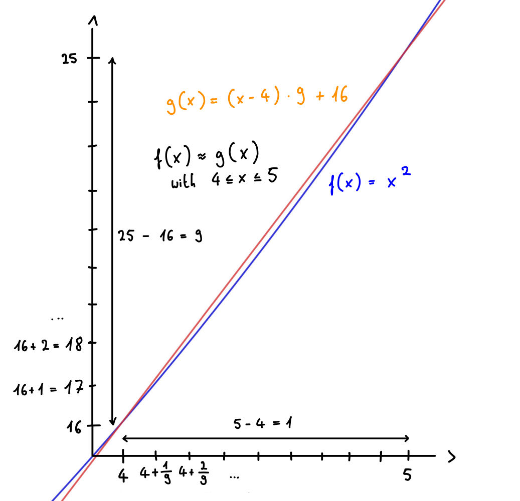
For example, what’s the square root of $17$? Not knowing how to algorithmically compute the best approximation of $\sqrt{17}$, we can make a pretty good intuitive guess by relying on our knowledge of square roots. We memorized that $\sqrt{16} = 4$, that the square of the next integer after $4$ is $5^2 = 25$ and that the function $f(x) = x^2$ is continuous. Based on this knowledge, we can quickly say that $\sqrt{17}$ must be somewhere in the lower part of the interval $[4, 5]$.
This gets us pretty far, but let’s keep going. To improve our guess without spending any time on (generally) random guesses, we can approximate $f(x)$ for $4 \leq x \leq 5$ as a linear function. Based on this, we can conclude that since $25 - 16 = 9$ and $\sqrt{25} - \sqrt{16} = 5 - 4 = 1$, $\sqrt{17} = \sqrt{16 + 1} \approx 4 + \frac{1}{9}$. All of these calculations can be easily performed in one’s head or quickly be scribbled down on a piece of paper. The figure below illustrates what I have just explained. Again, note that this doesn’t involve any calculations that are difficult to do by hand.
I hope you can see why this is so exciting! By simply memorizing of a few sample values and by internalizing the relationships of the operations we need through drilling, it’s possible to make very fast guesses about otherwise complex computations. To prove my point, let’s find out how close we got. $4 + \frac{1}{9} \approx 4.111$ and $\sqrt{17} = 4.123$: our guess was off by only $0.012$. Imagine if you could approximate something like $\log_{10}(64)$ just as quickly!
Powers, roots and logarithms
There is some confusion about the relationship between powers, roots, and logarithms. Some common operations such as addition and multiplication are commutative, unlike exponentiation, which is not. Commutativity means that $a + b = b + a$ and $a \cdot b = b \cdot a$: we can freely exchange the order of the operands. This is not the case with powers. Generally, $a^b$ is not the same as $b^a$ 2. We can show that exponentiation cannot be commutative by choosing an example that doesn’t fulfill this property: $3^4 = 81 \neq 4^3 = 64$.
The fact that exponentiation is not commutative makes it possible to define two methods of undoing exponentiation: the nth-root and the logarithm. This may seem surprising, since we’re so used to commutative operations like addition and multiplication that have only a single inverse operation.
Suppose we are given an exponentiation $x = b^n$ where $b$ and $x$ are positive real numbers, $b \neq 1$, and $n$ is a positive integer. If we know the values of $n$ and $x$, the nth-root gives the value of $b = \sqrt[n]{x}$. Otherwise, if we know the values of $b$ and $x$, the logarithm of $x$ to the base $b$ gives the values of the exponent $n = \log_b(x)$.
Both the nth-root and the logarithm take the result of an exponentiation as input. Simply put, what makes them different is the missing piece they fill in. Logarithms can be used to calculate the exponent from the result value and the base. The nth-root, on the other hand, takes the result value and the original exponent, to compute the base.
The following figure helped me personally to better understand the relationship between the three functions.
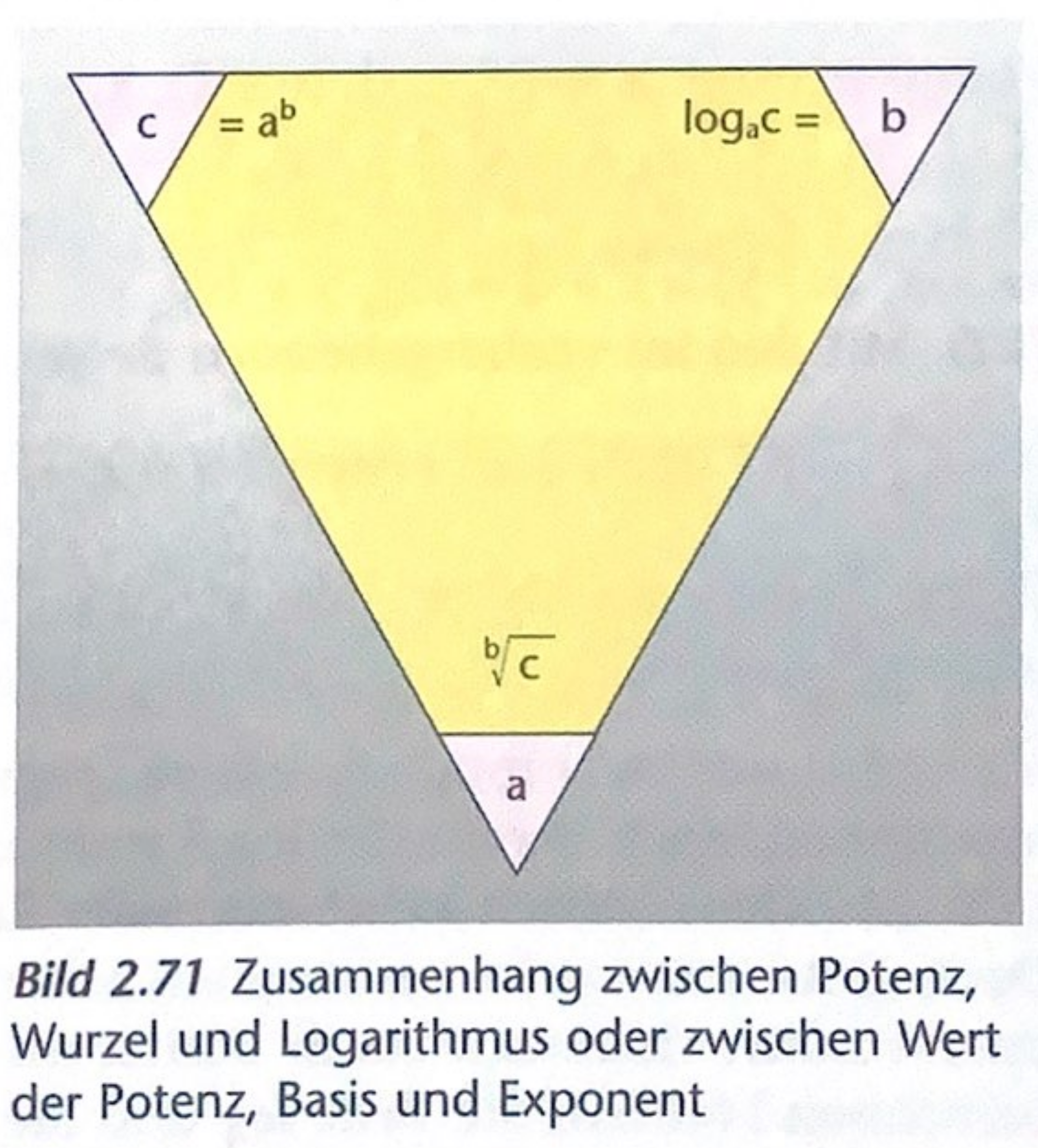
It comes from a German mathematics textbook called Handbuch Mathematik3 which translates to Handbook Mathematics. The caption reads: “Relationship between power, root and logarithm or between value of power, base and exponent”. This illustration shows the triangular relationship between the three functions, which is key. The same idea is used in this answer on Stack Exchange to suggest an alternative notation for powers, roots, and logarithms that emphasizes this relationship.
Definition of logarithms
Say we have an exponentiation $x = b^y$ where $y$, $b$ and $x$ are real numbers. From now on $b$ and $x$ are positive (excluding 0) and $b \neq 1$. For such an exponentiation, the logarithm of $x$ to the base $b$ is defined as
\[\log_b(x) = y ~~ \Leftrightarrow ~~ b^y = x\text{.}\]In the exponentiation $x = b^y$, if we know $x$ and $b$, the logarithm of $x$ to the base $b$ will give us the missing exponent. From this definition we get the following identities 4:
\[\text{(1)} ~~~ x = b^{\log_b(x)} ~~~~~~ \text{(2)} ~~~ x = \log_b({b^x})\text{.}\]Both of these are crucial. Ideally, you’d want them to come to mind every time you’re looking to solve a logarithmic equation. While they represent fundamental relationships of the logarithmic and exponential form, their reverseness makes them difficult to think about.
Let’s start by digesting $x = b^{\log_b(x)}$. To break up the equation, we’ll call the logarithm in the exponent $a = \log_b(x)$. This means that, $a$ is the exponent to the base $b$ such that $b^a = x$. With this step of indirection, it’s easy to see why the equation must be true. Think of it like this: “Raise $b$ to the power $a$ of $b$ that satisfies the property that $b^a = x$.”.
The second equation $x = \log_b(b^x)$ is easier to understand. I like to ask myself the question: “What’s the exponent $x$ to the base $b$, such that $b^x = b^x$? It’s $x$!”.
Based on this knowledge alone, we are also able to induce the values of a few logarithmic expressions. For example, what is the value of $\log_a(a)$? Since $a = a^1$, we can rewrite this as $\log_a(a^1)$ or equally $\log_a(a^x)$ with $x = 1$. Now, it’s obvious from the second identity that the answer is 1. The same approach of relying on the laws of exponents works for $\log_a(1)$. If we rewrite this in the same way by substituting $a^0$ for $1$, we get $\log_a(a^0) = 0$.
Multiplication as addition
The following is another central identity that opens up a lot of possibilities for us when it comes to computing logarithms manually.
\[\log_b(x \cdot y) = \log_b(x) + \log_b(y) ~~~~ \text{if} ~ y > 0\]The proof can be constructed from the two identities above and the rules of exponents. We start by using the first identity $x = b^{\log_b(b)}$ to substitute $x$ and $y$ in the left side of the equation:
\[\log_b(x \cdot y) = \log_b(b^{\log_b(x)} \cdot b^{\log_b(y)})\text{.}\]Using the law of exponents which states that $x^a \cdot x^b = x^{a + b}$, we can simplify this into
\[\log_b(b^{\log_b(x)} \cdot b^{\log_b(y)}) = \log_b(b^{\log_b(x) + \log_b(y)}) \text{.}\]Finally, the second identity $x = \log_b({b^x})$ is used to simplify this even further:
\[\log_b(b^{\log_b(x) + \log_b(y)}) = \log_b(x) + \log_b(y) \text{.}\]John Napier is said to have introduced this equation in 1614, and it quickly became famous because it allowed reducing complex multiplications to simple additions. Instead of performing the multiplication itself, people could simply look up the values of $\log_b(x)$ and $\log_b(y)$ and then add them together. This is one of the techniques we’ll use later to solve logarithmic equations by hand. Instead of looking up the values in a logarithm table, we’ll memorize a few key ones.
Division as subtraction
The laws of exponents also state that $x^a / x^b = x^{a - b}$. Hence, the above equation also works for division:
\[\log_b(x / y) = \log_b(x) - \log_b(y) ~~~~ \text{if} ~ y > 0 \text{.}\]Exponentiation as multiplication
There is another law of exponents which states that $(x^a)^b = x^{a \cdot b}$. Based on this, we get the following mind-boggling equation:
\[\log_b(x^c) = c \cdot \log_b(x)\]This can be proved by first defining an auxiliary variable $y = \log_b(x)$, so that $b^y = x$ (first identity). By substituting $b^y$ for $x$, we get \(\log_b((b^y)^c)\). Next, we apply this law of exponents:
\[\log_b((b^y)^c) = \log_b(b^{y \cdot c})\text{.}\]Lastly, we again apply the second identity from the definition and the substitute the original definition of $y$:
\[\log_b(b^{y \cdot c}) = y \cdot c = c \cdot \log_b(x)\text{.}\]Change of basis
This is the last concept we need to get started calculating logarithms by hand. The ability to change the base of a logarithmic expression is very valuable to us, because it means that we only have to remember a relatively small set of values for a single base. We’re then able to convert between bases and thereby solve expressions in a variety of bases.
\[\log_b(x) = \frac{\log_a(x)}{\log_a(b)} ~~~~ \text{if} ~ a > 0\]Again, we’ll start by defining a variable $y = \log_b(x)$. It’s important to recall that this is only used to simplify subsequent equations and make them easy to grasp. We can transform the left side of the equation into the exponential form.
\[\log_b(x) = y ~~ \Leftrightarrow ~~ b^y = x\]From here, we continue by taking the logarithm of both sides to the desired base $a$. Like $b$, $a$ can be any positive real number except $1$.
\[\begin{align*} b^y &= x & & | ~ \log_a\\ \log_a(b^y) &= \log_a(x) \end{align*}\]We can further transform this equation using the ‘exponentiation as multiplication’ identity.
\[\begin{align*} \log_a(b^y) &= \log_a(x)\\[2pt] y \cdot \log_a(b) &= \log_a(x) \end{align*}\]The final step is to isolate the variable $y$ and to substitute the original $\log_b(x)$ for it.
\[\begin{align*} y \cdot \log_a(b) &= \log_a(x) & & | ~ \div \log_a(b)\\[2pt] y &= \frac{\log_a(x)}{\log_a(b)}\\[2pt] \log_b(x) &= \frac{\log_a(x)}{\log_a(b)} \end{align*}\]It might be a good idea to make flash cards for yourself to memorize the different identities or rules we can use to transform logarithmic equations. Don’t put too much on the same card. Instead, try to spread out the different insights over several cards.
Theory-wise that’s all I am going to cover in this post. Obviously, there is a lot more to know about logarithms, which I have left out here for the sake of brevity. That said, all of this gives us a good foundation to expand on in the future. More importantly, it is enough for us to calculate the values of many different logarithmic expressions.
Memorize a logarithm table
As mentioned above, logarithms were a huge breakthrough when they were first discovered, because they made complicated calculations relatively simple. In a time before machine computers, this was very valuable. The values of many different logarithmic expressions were calculated once and then collected into so-called logarithm tables. After transforming a given problem, you could look up the closest value in the table, and you’d have a pretty good estimate.

Of course, memorizing that many numbers would be a bit extreme. It’s not impossible, and it will certainly improve the accuracy of your approximations, but it’s not worth the time for most people. Therefore, we will reduce the set of values to memorize to the bare minimum.
We can change the base of any logarithm to a base we know if we know the value of the logarithm of the original base to the desired base. This means that we only need to memorize a range of logarithms to a single base, as well as some logarithms of other bases to the same base we’ve chosen. Here, I opted for base $10$ logarithms and conversions from the natural and binary logarithms, since they are the most common. The range that we need to memorize is also quite small, since multiplications can be broken up into additions. That is, it’s sufficient to know the values of $\log_{10}(8)$ and $\log_{10}(10)$ to calculate $\log_{10}(80)$ because
\[\log_{10}(80) = \log_{10}(10 \cdot 8) = \log_{10}(10) + \log_{10}(8) \text{.}\]Depending on how hard you want to make it for yourself, you can also choose different degrees of precision. As suggested by kqr, it’s possible to get quite satisfactory results with only a single digit of precision. For completeness, I also added a higher precision option for each value. It makes sense to memorize the higher precision values for the logarithms that you’ll use most often. Therefore, the default precision for $\log_{10}(e)$ and $\log_{10}(2)$ is slightly higher.
| logarithm | base precision | base error | extra precision | extra precision error |
| $\log_{10}(1)$ | 0 | / | / | / |
| $\log_{10}(10)$ | 1 | / | / | / |
| $\log_{10}(e)$ | 0.43 | 1.00 % | 0.4343 | 0.00 % |
| $\log_{10}(2)$ | 0.30 | 0.34 % | 0.3010 | 0.01 % |
| $\log_{10}(3)$ | 0.5 | 4.80 % | 0.477 | 0.03 % |
| $\log_{10}(4)$ | 0.6 | 0.34 % | 0.602 | 0.01 % |
| $\log_{10}(5)$ | 0.7 | 0.15 % | 0.699 | 0.00 % |
| $\log_{10}(6)$ | 0.8 | 2.81 % | 0.778 | 0.02 % |
| $\log_{10}(7)$ | 0.8 | 5.34 % | 0.845 | 0.01 % |
| $\log_{10}(8)$ | 0.9 | 0.34 % | 0.903 | 0.01 % |
| $\log_{10}(9)$ | 1.0 | 4.80 % | 0.954 | 0.03 % |
As you can see, for each logarithmic expression there is a value with an error of less than 1 % (the one in green). Personally, I have chosen to memorize the following sequence of values. I find them relatively easy to remember because of their regularities. The downside of this is that some of the values have an error greater than 1 %. They also highlight a key characteristic of logarithmic growth, namely that the input value has to increase by some factor for the output value to increase by a constant amount5.
| $x$ | $e$ | 1 | 2 | 3 | 4 | 5 | 6 | 7 | 8 | 9 | 10 | ||||||||||||
| $\log_{10}(x)$ | 0.4343 | 0.0 | 0.3 | 0.5 | 0.6 | 0.7 | 0.8 | 0.85 | 0.9 | 0.95 | 1.0 | ||||||||||||
| $\underset{+0.3}{⤻}$ | $\underset{+0.2}{⤻}$ | $\underset{+0.1}{⤻}$ | $\underset{+0.1}{⤻}$ | $\underset{+0.1}{⤻}$ | $\underset{+0.05}{⤻}$ | $\underset{+0.05}{⤻}$ | $\underset{+0.05}{⤻}$ | $\underset{+0.05}{⤻}$ | |||||||||||||||
Again, I’d recommend you to create some flash cards for yourself to memorize these values. If you don’t care about precision that much, you can make it easier for yourself by using the more regular values in the lower table. Otherwise, use the upper table to pick and choose.
The hard part
Now we’ve got most things covered. The last piece that’s missing is getting it all into your brain forever. The best way to start is to look up a bunch of exercises and work through them. For example, I found this one early on.
I said at the beginning of this post that you’d learn how to quickly calculate $\log_{10}(64)$ by hand. Now that we have a good idea of what we’re dealing with, this shouldn’t be too difficult.
Let’s think: we need to break up $64$ into an expression made up of logarithms, we know. This is not difficult, for example $64 = 8 \cdot 8$. The rest is easy:
\[\log_{10}(64) = \log_{10}(8 \cdot 8) = \log_{10}(8) + \log_{10}(8) \approx 0.9 + 0.9 = 1.8\text{.}\]Just writing this, I am filled with a rush of excitement and awe. Let’s see how close we got this time. $\log_{10}(64) = 1.8062$ which means we were off by only $0.0062$! We won’t get this close for all numbers and many expressions are more difficult than this one. But to me, it’s really amazing how easy this is.
Above, I talked about the historical use of logarithms to speed up multiplications of large factors. Now we can use this technique as well. This answer on Stack Exchange is a good example of how to do so. Using logarithms in this way has become somewhat obsolete now that we have so many computers. But if you are interested in how to do this, you should definitely read the answer.
Finally, I want to show how we can use our newfound knowledge to solve for any exponent. For example, let’s look at the following equation: $0.5^x = 0.1$. Here, we have an unknown in the exponent. By definition, we need to use logarithms here.
\[\begin{align*} 0.5^x &= 0.1 & | ~~ \log_{0.5}\\[2pt] x &= \log_{0.5}(0.1) \end{align*}\]This time, we need to change the logarithm’s base to 10. After doing so, we are left with values which we have memorized.
\[\begin{align*} x &= \log_{0.5}(0.1)\\[2pt] x &= \frac{\log_{10}(0.1)}{\log_{10}(0.5)}\\[2pt] x &= \frac{\log_{10}(1 / 10)}{\log_{10}(1 / 2)}\\[2pt] x &= \frac{\log_{10}(1) - \log_{10}(10)}{\log_{10}(1) - \log_{10}(2)}\\[2pt] x &\approx \frac{0 - 1}{0 - 0.3}\\[2pt] x &\approx \frac{-1}{-0.3}\\[2pt] x &\approx 3.33 \end{align*}\]Conclusion
With this post, I hope to share some of the joyful moments of insight I felt as I delved deeper into understanding logarithms. Here, I have focused mainly on how to deal with logarithmic equations and how to solve them manually. There is much more to know about logarithms, about their history, their modern use, and especially their connection to the exponential function. Still, I have tried to provide comprehensive explanations, and I hope you found them insightful.
For one, many students dislike this sort of learning so much that they completely lose interest in math. ↩
In fact there are only two distinct numbers n and m that fulfill the requirement that $n^m = m^n$ which are $2^4 = 4^2 = 16$. ↩
Scholl, W., & Drews, R. (1997). Handbuch Mathematik. Falken. ↩
Knuth, E. (1997). The art of computer programming: Fundamental algorithms (3rd ed., Vol. 1). Addison Wesley Longman Publishing Co., Inc. ↩
Abelson, H., Sussman, G. J., & Sussman, J. (1996). Structure and Interpretation of Computer Programs (2nd ed.). Mit Press. 1.2.3 Orders of Growth ↩